
The springs and sticks model
A simple system that can learn any function with interesting physics!

In this blog, I will explain the springs-and-sticks model (introduced here), a simple but elegant regression model based on classical mechanics. This model combines ideas from machine learning and physics, and permits calculating interesting quantities such as the minimum energy required for learning a function (similar to the Landauer bound, but for regression).
Approximating functions with sticks
The springs-and-sticks (SS) model is a simple mechanical system composed (as its name suggests) of springs and sticks, and it performs regression using a mean-squared error loss. The idea behind it is the following: perform a piecewise linear approximation of a function with a stick-grid (this is similar to the trapezoidal rule, or to the functions parametrized by single-layer NNs with ReLU activation). Then we attach springs between the stick grid and the datapoints. We converge to the solution by dissipating the system’s energy, obtaining the best piecewise linear approximation (with constant spacing—although this can be relaxed) of the underlying function. Below, we show this method fitting a dataset sampled from a sinusoidal function:
It is clear to see that regression with this mechanical system is universal, as it can approximate any smooth function with a sufficiently fine grid (for a given epsilon, there is a grid spacing that achieves an error < epsilon). This model can be extended to any input and output dimension by adding more sticks and springs, respectively. The animation below shows this model for a 2D input.
Simulating the SS model
To simulate the dynamics of this model, we first define its Lagrangian and use the Euler-Lagrange equation to get the system’s equations of motion. We have developed a Python package that you can use to avoid implementing this step.
Instead of showing examples of our code, which can be found in the GitHub repository (github.com/bestquark/springs-and-sticks), let me explain the key points of the simulation:
The Lagrangian of this system is the difference between its kinetic energy and potential energy, obtained by summing the individual energies of each spring and each stick. For example, in the 1D piecewise linear approximation with N_s sticks of mass M, we have a kinetic energy of:
\( \begin{aligned} K_{\text{tr}} & = \sum_{i=0}^{N_s -1} \frac{1}{2} M v_i^2 =\frac{M}{8} \sum_{i=0}^{N_s -1} \left( \dot{x}_{i+1} + \dot{x}_i \right)^2, \\ K_{\text{rot}} &= \sum_{i=0}^{N_s -1} \frac{1}{2} I \omega_i^2 \approx \frac{M}{24} \sum_{i=0}^{N_s -1} \left( \dot{x}_{i+1} - \dot{x}_i \right)^2, \end{aligned}\)where x_i and x_{i+1} are the displacements of stick i’s extrema. For simplicity, the rotational energy uses the low-angle approximation of arcsine (this makes it easier to solve the EOMs while capturing the relevant dynamics we care about). The potential energy is the sum of the elastic energies of each spring (note that there is one spring per datapoint). The spring is attached between the datapoint “target” y_j and the model’s ‘prediction’ given by the linear interpolation between the ends of the underlying stick:
\(U_j = \frac{1}{2} k \cdot \delta_j = \frac{1}{2} k \cdot \left(\lambda_j x_i + (1-\lambda_j) x_{i+1} - y_j \right)^2 \)The corresponding EOMs obtained via Euler-Lagrange are non-dissipative. We model the dissipative behaviour using the Langevin equation, an equation with a dissipative term γ and random fluctuation term ξ. The strength of the fluctuations are dictated by the fluctuation-dissipation theorem: σ²=2 k_b T γ / M
\(\begin{aligned} \frac{d}{dt} \mathbf{x} &= \mathbf{\dot{x}}, \\ \frac{d}{dt} \mathbf{\dot{x}} &= {\mathbf{M}}^{-1} \mathbf{f}(\mathbf{x}, \mathbf{\dot{x}},t) - \gamma \mathbf{\dot{x}} + \sigma \dot{\mathbf{\xi}} (t). \end{aligned}\)To compute trajectories (over time), it is common to integrate stochastic differential equations with the “Euler-Maruyama” method (this is the standard Euler method of integration, but at each time-step we add the contribution of a random fluctuation). We use the torchsde package to solve this, getting the optimal “parameters” of the SS model once the system reaches a steady-state solution.
[Performance] Training the model on data
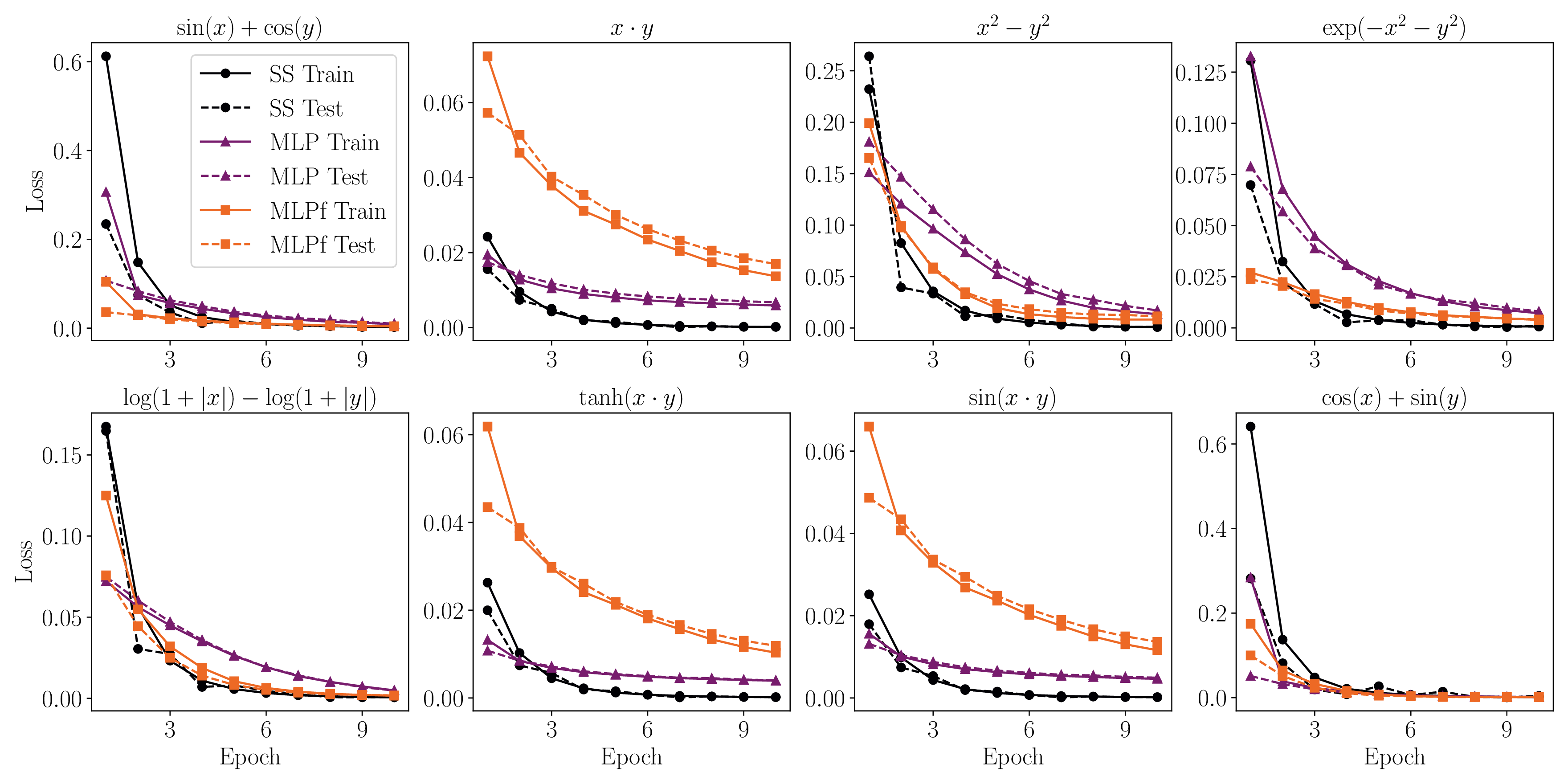
If you care about performance, you might be asking, is this model any useful for training on data? We show that it can learn smooth functions just as a single-layer neural network with ReLU activation functions (not a big surprise!). The main difference being that training is not achieved by gradient descent algorithms, but rather by time-evolving the dynamics of the SS model (which implicitly is doing gradient descent with momentum).
If you are familiar with diffusion models, you can think of the SS model as a diffusion model where x(0) → x(T) performs “training” instead of “interence”.
However, there is an important limitation with the current implementation of the model: the grid size grows exponentially in the input dimension (since the grid size has exponentially many points). This is a common problem faced in scientific computing, and common solutions include adaptive mesh refinement or multi-grid solvers. These or similar methods can alliviate this curse of dimensionality for the SS model.
[Thermodynamics] Making the system really small
Here is a thought experiment: suppose we make the SS system really really small, so small that the atoms in the environment hitting the sticks produce fluctuations so large that the system never converges to the “solution” of the regression problem1. This begs the question, is there a minimum energy scale for which the system cannot learn the underlying function? To answer this, we need to understand the relation of the energy the system dissipates vs. the “loss” of the model.
Given that the system is out of equilibrium, to compute this relationship we use the “Jarzynski equality” — which is a generalization of the second law of thermodynamics for non-equilibrium systems. This equality provides a way to compute the free-energy change from state A → B, by taking an average over many realizations of such process.
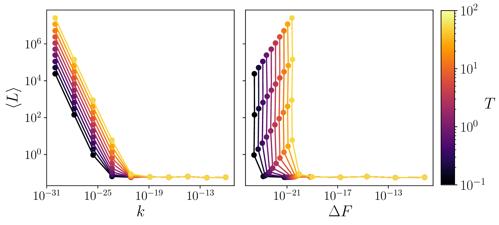
In our case, W is easy to compute since this is a classical mechanical system with well defined EOMs. We see that when the scale (k=M) is small enough, the model stops “learning” due to the low signal-to-noise ratio. This sets a minimum value for ΔF for which the model will not learn. We call this value a thermodynamic learning barrier (TLB). Below, we compute the TLB for multiple values of T:
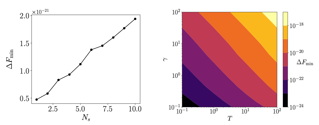
This TLB can be understood as a consequence of the fluctuation-dissipation theorem, where the fluctuations at a temperature T impose a minimum phase space volume V_f to which the system relaxes to. The TLB depends on parameters like the temperature, the dissipation constant in the EOMs, and in the amount of sticks (or “expressibility”) of the underlying model as shown below:
Could this open a way to understand scaling laws of neural networks from a physical point of view? I hope it does!
The full paper and the code are openly available:
Paper: https://arxiv.org/abs/2508.19015
Code: https://github.com/bestquark/springs-and-sticks
If you have any questions or feedback about this work, feel free to contact me at
luis (at) cs.toronto.edu
Stay curious!
Luis M.
Formally, these fluctuations happen around the solution, so taking many samples over time and averaging should give us the solution, but the “averaging” function requires dissipating energy (as its not a one-to-one map).