
Ranking Models for Bayesian Optimization

TL;DR—In self-driven molecular discovery, when you care about which molecules are best rather than how much better they are, train your Bayesian optimization surrogate to rank candidates instead of predicting exact values. In benchmarks spanning smooth and rugged chemical landscapes, rank‑based surrogates often match or beat standard regression models, especially early in the search and in the presence of activity cliffs.
Below, I will discussed the work presented in this article in detail.
The Challenge
Self-driving laboratories (SDLs) are a rapidly growing field in chemistry and materials science. In an SDL, automated experimental equipment (robots, flow reactors, etc.) is coupled with algorithms that choose which experiments to run next. The idea is to let a computer carry out the scientific loop: propose an experiment, execute it on the hardware, measure the outcome, and then update its plan.
A key challenge is in automated design of experiments, typically done using Bayesian optimization (BO). In BO, the goal is to maximize (or minimize) a black-box function – for instance, the yield or some property of a chemical reaction – with as few experiments as possible. The process works in a loop: the algorithm maintains a surrogate model of the unknown function, updates it with each new data point, and uses an acquisition function to pick the next experiment.
Running BO in chemical/materials problems comes with challenges. One major issue is data scarcity. Each experiment can be slow or costly, so initial datasets are often very small. Even though GPs are chosen for this regime, uncertainty remains high and the surrogate can be misleading with only a few points. Another issue is the roughness of chemical response surfaces. In many molecular and materials datasets, tiny changes in structure or composition can cause big jumps in a property, creating so-called activity cliffs. These cliffs make the underlying function “bumpy,” and difficult to learn for ML models. These challenges in building quantitative struture-activity relationship (QSAR) models results in unreliable optimization in SDL systems.
Ranking Over Regression
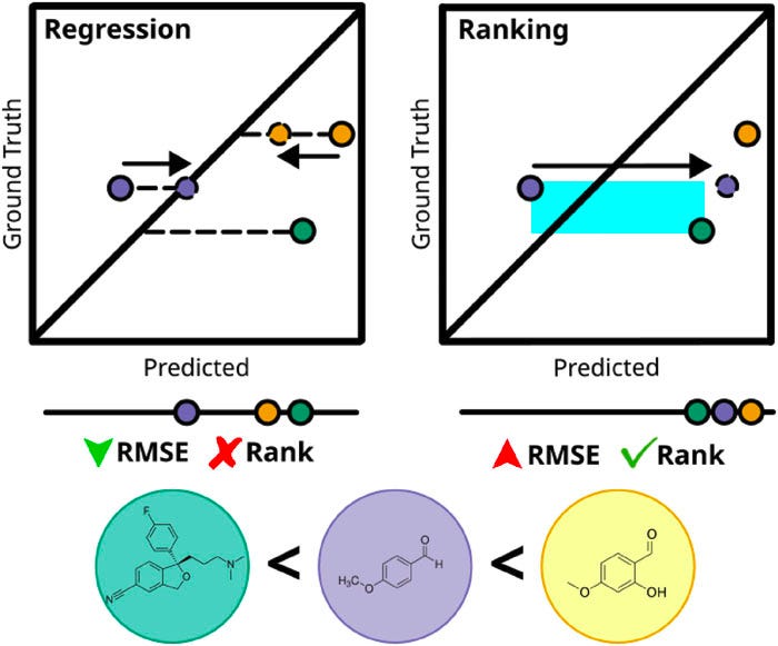
Imagine trying to rate every restaurant you’ve ever visited on a 1–10 scale. What does a “10” even mean? Is it your all‑time favorite taco truck... until you stumble on an even better birria tomorrow? And what’s a “1”—the worst meal imaginable, or just a bad night at a decent place? Without a shared sense of scale, those numbers float in space. You find yourself second‑guessing: Was that ramen a 7.5 or an 8? The scale is arbitrary, and—crucially—you don’t know where the true best or worst lie a priori.
Now switch the task: forget absolute scores and just answer, “Do I prefer restaurant A or B?” That’s suddenly easy. After enough A‑vs‑B choices, you can stitch together a remarkably stable personal ranking—your top five firms up, the middle shakes out, and the duds sink. And when a new spot opens, you don’t need to calibrate it on a 1–10 rubric; you only need to ask where it slots relative to places you’ve already tried. If it beats your current favorite, great—you’ve discovered a “better‑than‑10/10” without ever agreeing what “10/10” meant.
That’s the core intuition behind rank‑based Bayesian optimization (RBO) for molecular discovery. Traditional BO trains a surrogate model to predict numbers (regression): e.g., solubility, potency, or a multi‑property score. But in many discovery campaigns, what you really need is to pick the next candidate you’d test in the lab—more like choosing your next restaurant—so the relative order matters more than the exact value. RBO leans into that: it trains the surrogate on pairwise preferences (“molecule A is better than B”) and uses those learned rankings to steer the search.
So what does this mean in terms of molecule selection?
Ranking is easier. Rather than learning the high-dimensional and complex QSAR of molecules to properties, ranking models learn the relative ordering of molecules in terms of their pairwise preferences, which aligns better with our ultimate goal of BO in SDLs: finding the best candidate molecules! This simplifies the problem for the model at the expense of a less informative (or less “knowledgeable”) and less interpretable surrogate model.
Robust to cliffs and outliers. Activity cliffs make regression hard: a few extreme points can pull the scale around, leading to large losses that affect the training of regression models. And more importantly, these outliers may very well be the optimal molecules we are seeking. If the regression model manages to minimize the average root mean squared errors (RMSE), it would all be for naught if it didn’t get the relative ranking correct.
No scale? No problem. Early in a campaign you don’t know what “best‑possible” looks like. Ranking asks only for relative judgments, which are easier to learn reliably from limited data—just like deciding A vs B is easier than inventing an absolute score.
The Experiment
We can directly show the effect of using RBO by simulating an SDL campaign. Using some select datasets, we can run many molecular selection campaigns to gather statistics and evaluate the performance of regression BO and RBO for direct comparison.
What models are we using as surrogates?
Deep learning models: multi-layer perceptron (MLP), Bayesian Neural Network (BNN), Graph Neural Network (GNN with variational last layer).
Regression models use the standard mean squared error (MSE).
Classic baseline: Gaussian Process (GP) with a Tanimoto kernel on ECFP fingerprints.
What is the loss function for ranking models?
Pairwise margin ranking loss on sampled pairs. The loss takes in pairs of data points, mapping it to a scalar loss value:
2N pairs are sampled each BO iteration for tractability; pairs are resampled between iterations. The ranking model outputs scores whose relative differences matter (they are not calibrated property predictions).
What are the datasets?
ZINC‑derived sets (2,000 molecules each) with 12 objectives (e.g., GuacaMol benchmarks, LogP, QED). These are derived following the work of Aldeghi et al., who use these different objectives to study the roughness of molecular datasets, measured by the Roughness Index (ROGI).
MoleculeACE datasets from ChEMBL with activity cliffs, curated by van Tilborg et al. for studying the effect of highly rugged functional spaces in drug activity prediction. The curated datasets involve the minimization of the inhibitor constant KiKi (the concentration required for half-maximal inhibition of a target protein) and the half-maximal effective concentration EC50EC50 (the concentration required for half-maximal response of the drug), both of which measure the effectiveness of drug molecules.
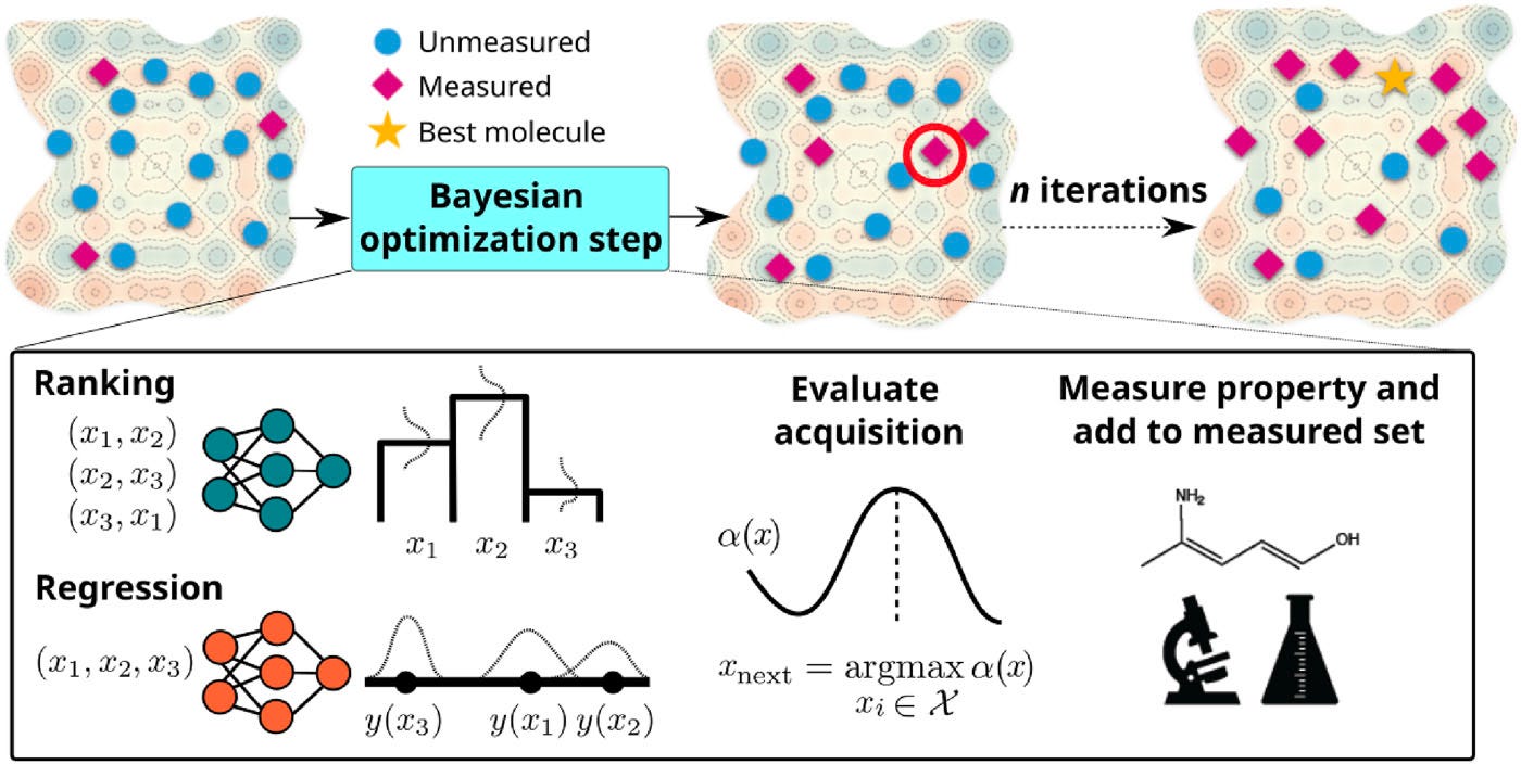
Bayesian optimization loop
The BO loop is shown in Figure 2. At its core, BO employs the surrogate model to learn from previously evaluated molecules to predict the properties of unexplored candidates. Because the properties are already provided by the datasets, the experimental “measurement” is a lookup of the respective properties in the datasets.
The optimization starts with an exploration phase, where 10 random molecules are selected from the dataset to establish a baseline understanding of the chemical space. The algorithm proceeds through 100 additional iterations, creating a total budget of 110 simulated measurements.
At each iteration, the surrogate model is trained on the current “measured set” of molecules, learning to predict either property values (in regression-based BO) or relative rankings (in RBO) for the remaining unexplored molecules. The acquisition function serves as the decision-making engine of the optimization process, determining which molecule to measure next by balancing exploration of uncertain regions with exploitation of promising areas. For probabilistic models like Bayesian neural networks, graph neural networks, and Gaussian processes, the Upper Confidence Bound (UCB) acquisition function is employed, defined as
where ŷ represents the predicted mean, 𝜎̂ the uncertainty, and β = 0.3 controls the exploration-exploitation trade-off. This formulation ensures that molecules with high predicted values or high uncertainty receive priority, encouraging both exploitation of promising candidates and exploration of under-sampled regions. For deterministic models like the MLP, a greedy selection approach is used, where the molecule with the highest predicted value is chosen directly.
After selecting the next molecule, the algorithm simulates its property measurement and adds it to the measured set. The surrogate model is then retrained on this expanded dataset, incorporating the new information to improve future predictions. This iterative process continues until the evaluation budget is exhausted, with each iteration refining the model’s understanding of the structure-property relationships in the chemical space.
Metrics of success
To measure the success of the optimization process, we use the Area-Under-Curve (AUC) of the fraction of top-100 molecules found versus the number of evaluations. This metric rewards methods that identify high-performing candidates early in the optimization process. This metric is dubbed BO-AUC.
Uncertainty calibration also plays an important role in Bayesian optimization, as acquisition functions rely on both predicted means and uncertainties to balance exploration and exploitation. A well-calibrated model should produce uncertainty estimates that accurately reflect prediction confidence—when the model claims high uncertainty, predictions should indeed be less reliable. For regression models, we evaluate calibration using the standard regression expected calibration error (rECE), which measures how well the predicted uncertainties match the actual prediction errors. For ranking models, we devised the pairwise-ranking expected calibration error (prECE), which assesses calibration by comparing the fraction of correctly ranked pairs to the model’s ranking confidence across different confidence bins. The prECE is defined as:
where P is the set of all unique pairs, M is the number of confidence bins (set to 10), Bm contains pairs with ranking confidence in bin m, I(yi>yj) is the indicator function for correct ranking, and P(ŷi>ŷj) is the model’s ranking confidence, defined as:
where Φ is the standard Gaussian cumulative distribution function. Notice that when z>0, the model predicts that yi>yj with P>0.5 and vice versa for z<0. When z→0, which occurs when the ranking scores are close and the uncertainties are high, (ŷi−ŷj)2≪𝜎̂i2+𝜎̂j2, the probability approaches 0.5 and the model has low confidence in the prediction.
Key Findings
1) Ranking surrogates are more robust in rough landscapes
Figure 3. BO-AUC vs dataset roughness (ROGI) on ZINC tasks. Ranking-trained deep surrogates (BNN/MLP/GNN) maintain higher BO-AUC than regression counterparts as roughness increases, and are competitive with a GP baseline on smoother sets.
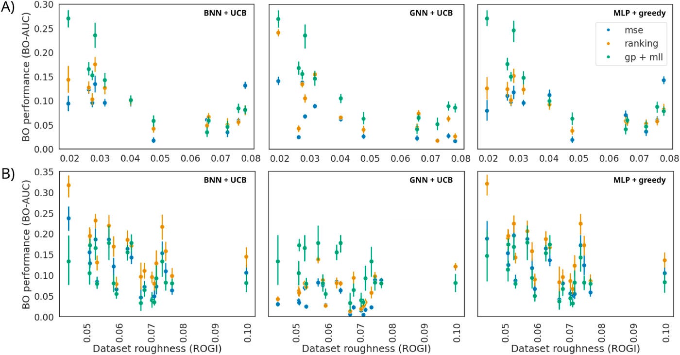
In Figure 3, we plot the BO performance for each of the ZINC tasks as a function of the ROGI of the dataset. The performances are shown for the regression DL surrogates, their ranking counterparts, and the GP surrogate. Across the ZINC tasks, ranking-trained deep models often achieve higher BO-AUC than their regression-trained counterparts, finding more of the top-100 molecules sooner.
Performance degrades as dataset roughness (measured by ROGI) increases for all surrogates, but ranking models handle this degradation more gracefully than regression models. GPs remain strong on smoother datasets, while ranking-trained deep models become competitive on rougher ones. Overall, the results show similar or improved performance with ranking surrogate models.
2) Ranking models perform better on activity cliffs
Figure 4. MoleculeACE (activity-cliff) results: fraction of datasets where ranking training beats, ties, or trails regression and the GP. Ranking improves BNN/MLP and narrows the gap for GNNs.
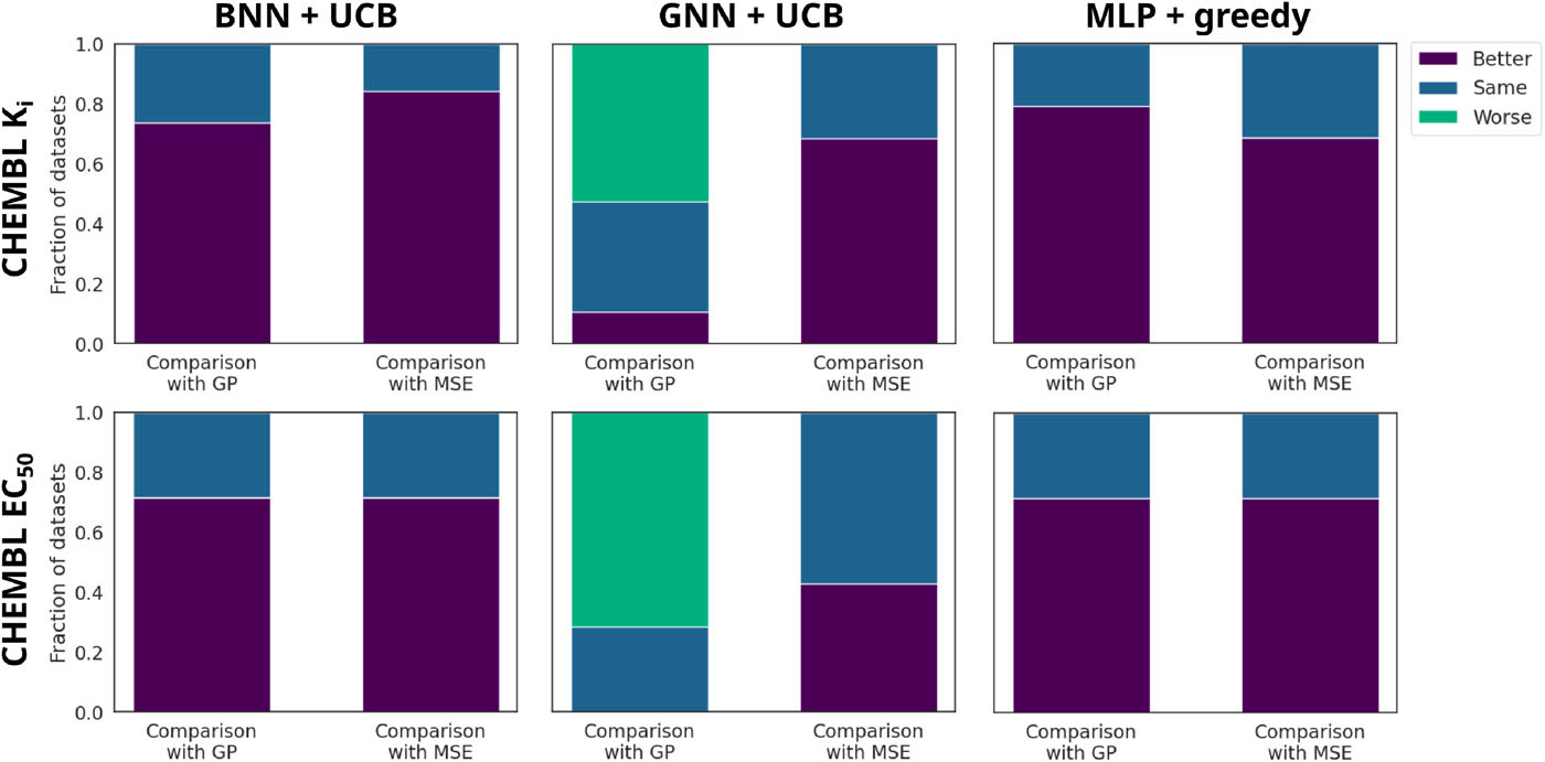
On MoleculeACE datasets—which are rich in activity cliffs—ranking models frequently outperform their regression counterparts and often match or exceed GP performance for BNN and MLP surrogates. In Figure 4, we show the fraction of datasets in which the ranking models peform better, the same, or worse than their regression counterparts and the GP surrogate. While GNNs still struggle overall on these challenging datasets, ranking training consistently improves their performance over regression training. Statistical tests across all datasets confirm these trends, with ranking models winning on more datasets than they lose.
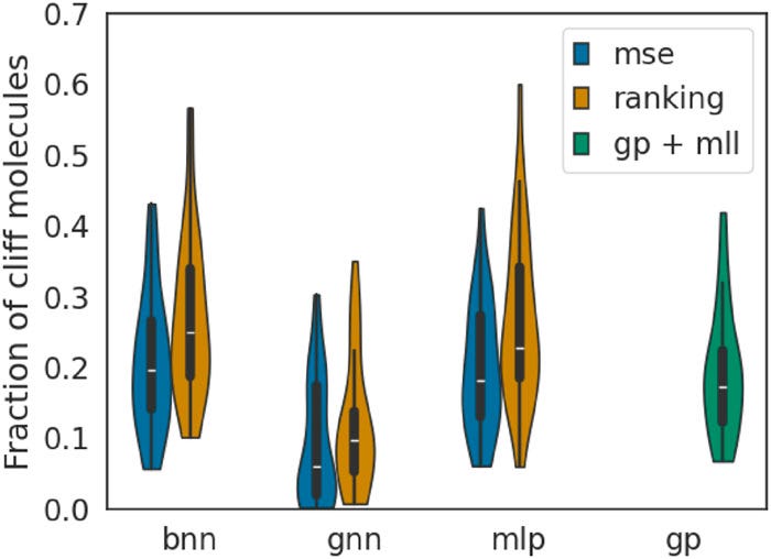
As defined by van Tilborg et al., activity cliffs in the MoleculeACE datasets are labelled by cliff-pair molecules. To see how well the surrogates handle the activity cliffs, we look at the fraction of top-100 molecules discovered by our surrogate models. The violin plots in Figure 5 reveal that ranking models identify a larger fraction of cliff molecules among the true top-100 candidates, demonstrating their ability to navigate the discontinuities where optimal molecules often reside.
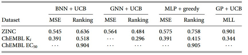
3) What metric correlates with BO success? Ranking quality, not R²
We tracked surrogate test-set performance throughout the BO campaigns and found that Kendall’s τ (rank correlation) positively correlates with BO outcomes, while R² shows no reliable relationship—even for GP regressors. These statistics are shown in Table 1. The correlations are particularly strong for ranking models: BNN ranking shows τ = 0.636 on ZINC datasets and τ = 0.518 on ChEMBL Ki datasets, while regression models show weaker or non-significant correlations.
Ranking models achieve useful τ values earlier in the optimization loop (iteration 1) and maintain advantages through iteration 100 in many settings. This early ranking capability helps explain why they front-load discoveries, leading to higher BO-AUC scores.
4) Uncertainty calibration matters—but accuracy matters more
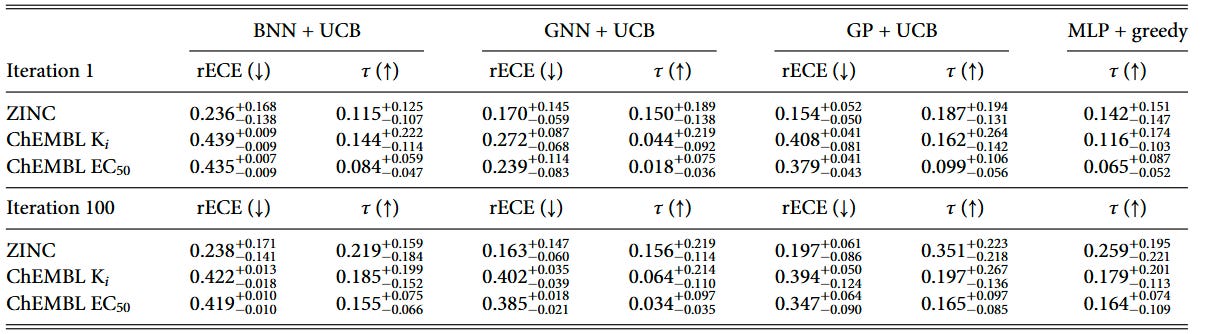
Throughout the BO campaign, we monitor the calibration and ranking ability on a held-out test set. To show the change in the model ability, we show the metrics for the first and last iterations of the BO campaign in Tables 2 and 3.
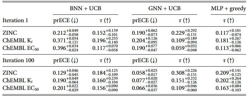
We introduced pairwise ranking ECE (prECE) to gauge calibration for ranking surrogates, analogous to rECE for regression models. Calibration improves with more data for both model types, but consistent with prior work by Foldager et al., better calibration alone doesn’t guarantee better BO performance. Ranking accuracy (as measured by Kendall’s τ) proves to be the stronger driver of optimization success.
The calibration analysis shows that ranking models achieve relatively low prECE values, particularly in later iterations, while regression models generally have higher calibration errors due to poor predictive performance in low-data regimes. This reinforces that while calibration is important, the fundamental ability to rank candidates correctly is what ultimately drives BO success.
Practical guidance for practitioners
When to use what:
Smooth landscape and very little data: start with a GP and an appropriate kernel.
Rough or unknown landscape, or signs of activity cliffs: try a ranking‑trained deep surrogate (BNN or MLP). Expect better early ordering, not necessarily better absolute predictions.
If you need calibrated numeric predictions later (constraints, safety): keep or switch to regression once data grow; ranking often remains competitive for selection.
Implementation notes:
Pairwise margin ranking loss can have an enforced margin (a minimum gap between the scores), here we use zero margin for a pure ranking problem.
Representations: ECFP (2048, r = 3) for MLP/BNN; GP with a Tanimoto kernel on ECFP is a strong baseline.
Acquisition: UCB with β ≈ 0.3 worked reliably; EI showed similar trends.
Monitor Kendall’s τ each iteration; in these settings it tracks BO progress better than R².
Limitations
Limited tuning: settings mirror low‑data workflows; more tuning or different representations could change results.
Compute/memory: pairwise training adds cost; usually minor vs. lab time but relevant in tight loops or large simulations.
Only pairwise comparisons considered: there are many other ranking losses that involve more ordered sets, such as list-wise, or triplet losses. These losses may be more efficient or effective, however we do not study them here.
Noise: high experimental noise can blur pairwise labels; replicates or robust losses may help.
Multi‑objective scope: this work is single‑objective; use scalarization or Pareto methods for multiple objectives.
Bottom line
RBO shifts focus from predicting calibrated values to getting the order right. In molecular BO, this can speed early discovery in rugged or low‑data settings. GPs are a strong choice on smooth problems; ranking‑trained deep surrogates are a practical alternative when cliffs, noise, or limited data are likely. Choose based on your objective and constraints.
Most people are still optimising tools.
My work has been to rebuild the operating system.
For almost three decades I’ve been working in a space that is structurally invisible: not on the next app, but on the logic by which civilizations think, decide and orient themselves under complexity and AI.
No institutional think tank.
No corporate innovation lab.
Just persistent, long-range research across media theory, systems thinking, AI and governance that has crystallised into a field I call Ontocybernetics – the study and design of how being, knowing and governing are coupled in a digitised world.
From this, three core frameworks emerged:
• Sapiognosis – cognition as orientation, not accumulation.
• Sapiopoiesis – systems that enable becoming, not just survive.
• Sapiocracy – governance as coherence, not power.
Together they form the Epistemic Integrity Umbrella:
• an Epistemic Core that decides what can count as relevant, viable and responsible in the first place,
• an Orientation Layer that protects subject autonomy and judgment under complexity,
• and a design logic for aligning human and AI systems without collapsing everything back into control and extraction.
If you sense that
• incremental “AI ethics” is no longer enough,
• current institutions run on obsolete epistemic grammars,
• and the real leverage lies in the conditions of judgment, not in yet another framework deck –
then you are exactly the kind of mind this is built for.
My Substack is not a newsletter.
It is the primary lab and publication channel for this work: serialized essays, conceptual maps, and the emerging blueprint of a sapiopoietic civilization – written for people who design systems, not slogans.
Those who join as founding members are what I call the Minds of Integrity:
an inner circle who help anchor a genuinely human-centred future at the level of the epistemic core – where orientation, not noise, will decide what our technologies and institutions become.
If you want maximum impact with minimal noise, this is one of the few places where supporting a single project has structural leverage – more effect than a thousand well-meant but redundant initiatives that cancel each other out.
👉 Become a supporter or founding member here:
https://leontsvasmansapiognosis.substack.com/subscribe
If the future needs anything, it is not more content –
it is a coherent epistemic core, with Minds of Integrity to guard it.
That is what I have been building.