HIP: Hessian Interatomic Potentials

Reaction rates, SE(3)-equivariant matrices, and how Hessians improve energies and forces.

Until recently, fast and accurate Hessians have eluded us.
With HIP, we can now directly predict Hessians, orders of magnitude faster and more accurate than autodiff or finite difference. All we need is a small readout head on top of our favourite MLIPs.

HIP: a regular MLIP (dark) with the right readout head (green) enables fast and accurate Hessians

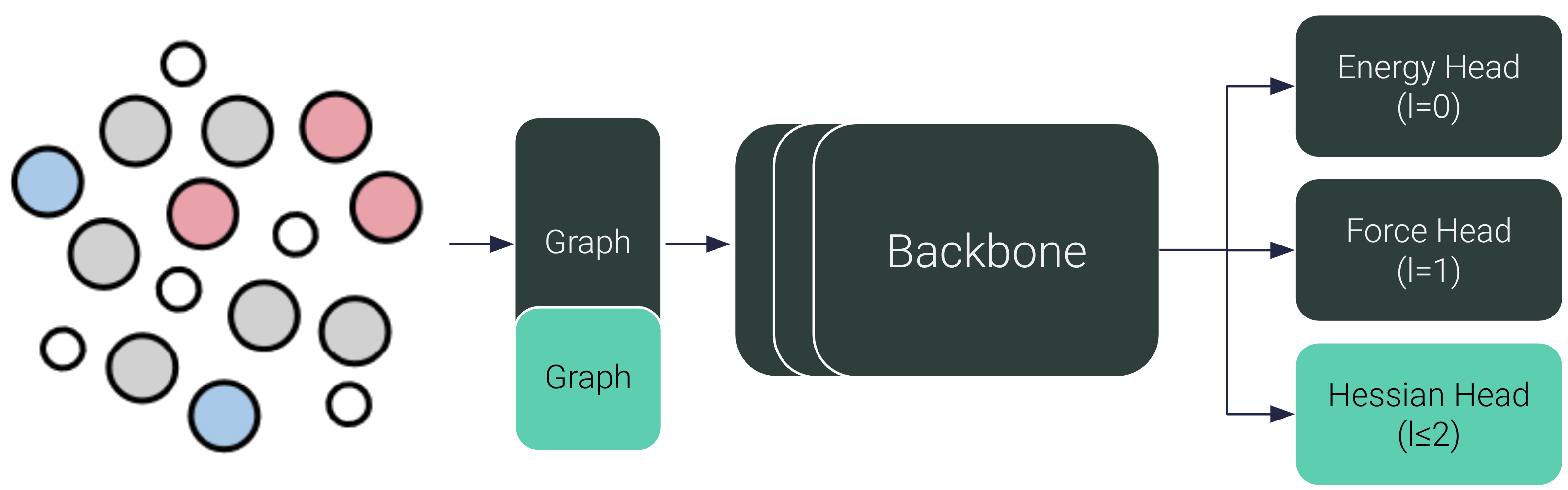
In this blog post we go into the importance of Hessians for reaction rates, and how we can construct the Hessian to be SE(3)-equivariant and symmetric by design. At the end, we present yet unpublished results: HIP also improves energy and force predictions.

What Hessian are we talking about?

Electronic-structure methods (like DFT), classical force fields, and machine-learning interatomic potentials (MLIPs) all aim to do the same thing: given atomic positions R and atom types Z, predict an energy E (and the forces).

\(E = E(\mathbf{R}, \mathbf{Z}) \in \mathbb{R}\)

\(\mathbf{R} = (\mathbf{r}_1, \dots, \mathbf{r}_N) \in \mathbb{R}^{3N} ,\quad \mathbf{Z} = (Z_1, \dots, Z_N)\)

The forces are the first derivatives of the energy w.r.t. positions:

\(\mathbf{F} = -\frac{\partial E}{\partial \mathbf{R}} \in \mathbb{R}^{3N}.\)

Often we also need the **second** derivatives, i.e. the (massive) 3Nx3N Hessian:

\(H_{;i\alpha,, j\beta} = \frac{\partial^2 E}{\partial R_{i\alpha}, \partial R_{j\beta}} \in \mathbb{R}^{3N \times 3N} ,\quad \alpha,\beta \in {x,y,z}\)

where i,j = 1,…,N index atoms and Greek symbols index Cartesian components.

In DFT, this nuclear Hessian can often be computed analytically, but it is expensive. With HIP, we show how to obtain that very Hessian from an MLIP.

Note: in optimization of neural networks you may also see a different Hessian, which is the second derivative of the loss w.r.t. weights. That Hessian is used to speed up training. Here we are talking about the Hessian of the potential energy w.r.t. atomic coordinates. But similarly, we can later use our Hessian to optimize geometries faster to a low energy configuration.

Why Hessians?

Chemical reactions from transition states

Beyond geometry optimization, the most important use of Hessians in chemistry is computing reaction rates with transition state theory.

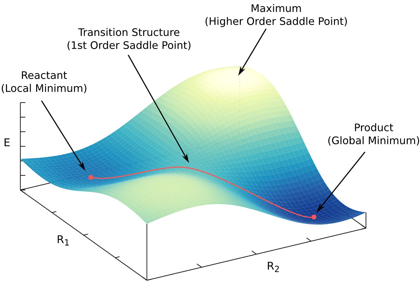
Physical systems prefer low-energy, stable states (think of the Boltzmann distribution: states with lower energy are more populated). Occasionally, a system crosses from one stable state to another, for example, a chemical reaction. The highest point in energy along that path is the transition state (TS).

Reactions are hard to simulate because there are many possible paths from reactant A to product B, and in principle we should sample all of them (see transition path sampling). A very effective simplification is to focus only on A, B, and the transition state that connects them.

Credit: Combining Machine Learning and Computational Chemistry for Predictive Insights Into Chemical Systems

Transition states are identified by the Hessian

We need the Hessian because a transition state is a saddle point. Minima, maxima, and saddle points all have zero gradient; the only way to tell them apart is by the curvature, i.e. the Hessian.

A proper transition state is a saddle point of index 1. That means: the Hessian has exactly one negative eigenvalue (equivalently, exactly one imaginary vibrational frequency). Most TS-search methods also follow the eigenvector associated with that lowest eigenvalue to locate the TS.

So, to find and to confirm a transition state, we need the Hessian.

More Hessian in calculating reaction rates

Once we have the TS, the Hessian shows up again in the rate calculation.

In transition state theory, the rate constant k is usually written in the Eyring form, in terms of the Gibbs free-energy barrier.

\(k = \frac{k_B T}{h} \exp\!\left( - \frac{\Delta G^\ddagger}{R T} \right) \)

The activation free energy is the Gibbs energy of the transition state minus of the reactant.

\(\Delta G^\ddagger = G_{\text{TS}} - G_{\text{reactant}}. \)

\(\Delta G^\ddagger = \Delta E_{\text{elec}} + \Delta E_{\text{ZPE}} + \Delta H_{\text{thermal}} - T \, \Delta S_{\text{thermal}}\)

To get that Gibbs energy, we need vibrational frequencies from the Hessian (which you get from the eigenvalues after mass-weighting).

\(\mathbf{F}_{ij} = \frac{ \mathbf{H}_{ij} }{ \sqrt{m_i m_j} } ,\quad \mathbf{F} \mathbf{L} = \mathbf{L} \mathbf{\Lambda} ,\quad \mathbf{\Lambda} = \mathrm{diag}(\lambda_1, \lambda_2, \dots, \lambda_{3N-6}) , \quad \nu_k = \frac{1}{2 \pi} \sqrt{\lambda_k}\)

Those frequencies give us the zero-point energy, because nuclear vibrations are quantized and have a nonzero energy even at absolute zero.

\(E_{\text{ZPE}} = \frac{1}{2} \sum_i h \nu_i\)

The Gibbs energy change also depends on the enthalpy change, which again is built from temperature-corrected vibrational contributions, so, again, Hessian frequencies.

\(\Delta H_{\text{thermal}}(T) \propto \Delta H_{\text{vib}}(T) = \sum_{i=1}^{3N-6} \left[ \frac{1}{2} h \nu_i + \frac{h \nu_i}{\exp\!\left( \frac{h \nu_i}{k_B T} \right) - 1} \right] \)

Even the entropy term S includes vibrational parts.
In short: for accurate reaction rates, Hessians are everywhere.

How to construct a Hessian (in theory)

Hessians obey two key symmetries: (1) they are symmetric under transpose and (2) they are SE(3)-equivariant under rotations.

One 3x3 block at a time

It’s helpful to view the Hessian as an NxN matrix of 3x3 blocks. Each block describes the coupling between atoms i and j (or the self-term when i=j). Since atomic positions live in (x,y,z), each block is

\(H_{ij}= \frac{\partial^2 E}{\partial \mathbf{r}_i \partial \mathbf{r}_j}= \frac{\partial^2 E}{\partial \mathbf{r}_j \partial \mathbf{r}_i}\in \mathbb{R}^{3\times 3}, \quad\mathbf{r} = (x,y,z)^\top, \quad i,j=1,\dots,N\)

Under a global rotation Q, every 3x3 block must itself transform like a rank-2 Cartesian tensor (a.k.a. a matrix, in the linear algebra sense, not the computer science 2D-array sense):

\(H_{ij} \mapsto Q, H_{ij}, Q^\top\)

The fact that each 3x3 block behaves like a separate matrix, makes it easier to talk about how construct one block at a time than looking at the whole Hessian.

What follows is how to construct each such 3x3 block, so that the symmetries are built in. The math is hard, but the code is easy! The rest of this section compiles down to just 16 lines of code:

def irreps_to_cartesian_matrix(irreps: torch.Tensor) -> torch.Tensor:
    “”“Luca Thiede’s creation.
    irreps: torch.Tensor [N, 9] or [E, 9]
    Returns:
        torch.Tensor [N, 3, 3] or [E, 3, 3]
    “”“
    return (
        einops.einsum(
            o3.wigner_3j(1, 1, 0, dtype=irreps.dtype, device=irreps.device),
            irreps[..., :1],
            “m1 m2 m3, b m3 -> b m1 m2”,
        )
        + einops.einsum(
            o3.wigner_3j(1, 1, 1, dtype=irreps.dtype, device=irreps.device),
            irreps[..., 1:4],
            “m1 m2 m3, b m3 -> b m1 m2”,
        )
        + einops.einsum(
            o3.wigner_3j(1, 1, 2, dtype=irreps.dtype, device=irreps.device),
            irreps[..., 4:9],
            “m1 m2 m3, b m3 -> b m1 m2”,
        )
    )

From spherical features to 3x3 tensors

Equivariant networks based on spherical harmonics store features as coefficients of irreducible representations (irreps) of SO(3). For SO(3), irreps are labelled by l=0,1,2,… . The l-th irrep has 2l+1 entries with basis m=-l,…,+l. These are the same (\ell)’s as in angular momentum and in the spherical harmonics: When rotating each l rotates separately, via their Wigner-D matrix, never across different l’s. That is the irreducibility.

In practice, most MLIPs use l up to around four. Here we only need l up to two.
The first 9 channels of a node/edge feature store exactly this:

\([\underbrace{a^{(0)}}_{1} | \underbrace{a^{(1)}_m}_{3} | \underbrace{a^{(2)}_m}_{5} ] \in \mathbb{R}^9\)

Our goal is to turn these spherical pieces into a Cartesian 3x3 tensor. The key observation is

\(1 \otimes 1 = \underbrace{\text{scalar}}_{\ell=0} \oplus \underbrace{\text{antisymmetric}}_{\ell=1} \oplus \underbrace{\text{symmetric traceless}}_{\ell=2},\)

So the tensor product of two vector irreps l=1 (a matrix) decomposes into the l=0,1,2 content that we have. Concretely, we want a matrix M in the spherical-(1) basis

\(M_{m_1 m_2}, \quad m_1,m_2\in{-1,0,1}\)

Visualizing the transformation

Before jumping into the math, a helpful way to look at this 3x3 block construction is to see the role of each irrep:

Credit: A Hitchhiker’s Guide to Geometric GNNs for 3D Atomic Systems

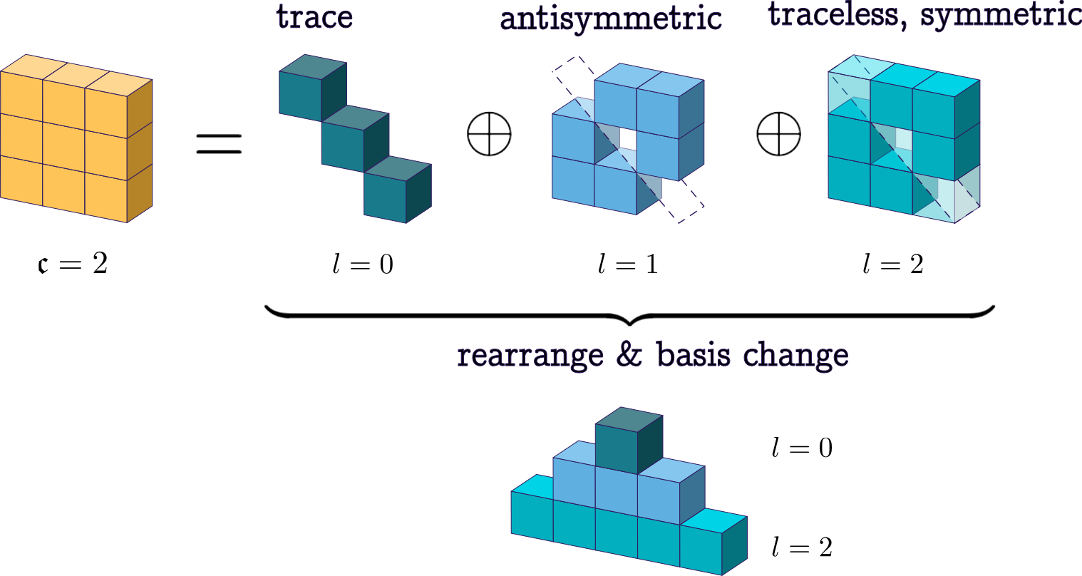
The l=0 slice, which consists of just one number, becomes the isotropic component, the trace part of the tensor. The l=1 slice, which has three components, becomes the antisymmetric part and can be written as the skew-symmetric matrix

\([\mathbf{v}]\times =\begin{pmatrix}0 & -v_z & v_y \\ v_z & 0 & -v_x \\ -v_y & v_x & 0\end{pmatrix}\)

so it encodes the axial or pseudovector content. The l=2 slice, which has five components, becomes the symmetric traceless part S. Altogether, the resulting Cartesian tensor can be written as:

\(1 \otimes 1 = \underbrace{\text{scalar}}_{\ell=0} \oplus \underbrace{\text{antisymmetric}}_{\ell=1} \oplus \underbrace{\text{symmetric traceless}}_{\ell=2}\)

which is precisely the general decomposition of a 3x3 tensor.

Enter Clebsch–Gordan / Wigner 3j

In physics speak, building the 3x3 matrix is the same going from the coupled basis to the uncoupled basis. Coupling and decoupling angular momenta is done by Clebsch–Gordan (CG) coefficients. Wigner 3j symbols contain the same information, just symmetrized and differently normalized:

\(\underbrace{ \begin{pmatrix} j_1 & j_2 & J \\ m_1 & m_2 & -M \end{pmatrix}}_{\text{Wigner 3j}} = \underbrace{\frac{(-1)^{j_1 - j_2 + M}}{\sqrt{2J+1}}}_{\text{phase & normalization}} \underbrace{\langle j_1 m_1, j_2 m_2 \mid J M\rangle}_{\text{Clebsch–Gordan}} \)

The minus sign in the third (m) makes the 3j symbol nicely symmetric, which is why it’s convenient for einsums.

Using these 3j symbols, we couple each l-slice to produce the 3x3 spherical-basis tensor:

\(M_{m_1 m_2}= \sum_{\ell=0}^2 \sum_{m=-\ell}^\ell\begin{pmatrix}1 & 1 & \ell \\ m_1 & m_2 & m\end{pmatrix}, a^{(\ell)}_m\)

The triangle rule and m1+m2+m=0 enforce that the output transforms correctly.
That double sum is exactly what this einsum does:

“m1 m2 m3, b m3 -> b m1 m2”

where “m1 m2 m3” is the precomputed 3j tensor for each l, and “b m3” is the batch of l-features. We do the contraction for l=0,1,2 and sum them up:

\(M = \bigl( \text{3j}_{\ell=0} \,\circledast\, a^{(0)} \bigr) + \bigl( \text{3j}_{\ell=1} \,\circledast\, a^{(1)} \bigr) + \bigl( \text{3j}_{\ell=2} \,\circledast\, a^{(2)} \bigr).\)

combined these are exactly the 16 lines of code above.

Phew, that was a lot.

Assembling the Hessian

We now saw how to compute the 3x3 blocks from spherical harmonic features. The question we haven’t answered yet is where we get the spherical harmonics features from. We chose the simplest route:

(1) The diagonal entries of the Hessian are just the self-interaction of an atom with itself. For these, we just use the features on each nodes as is.

(2) The off-diagonal entries of the Hessian are the interaction between two different atoms. We already have the machinery for learning interactions: message passing. We compute messages (“edge features”) between the atoms, and use them directly instead of summing or otherwise aggregating them.

The arrangement of 3x3 blocks in the Hessian are depicted in this figure:
We turn the node features (circles) and messages on the edges (arrows) into the diagonal and off-diagonal entries of the Hessian. Each colour in the Hessian is itself a 3x3 block.

How the HIP readout assembles node features (circles) and edge features (arrows) (left) to the Hessian (right). Node features become diagonal entries, messages on the edges become off-diagonal entries. Each coloured block has 3x3 entries.

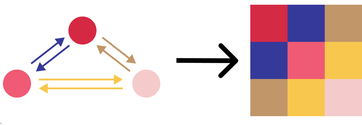
So, from the individual 3x3 blocks, we can assemble the full Hessian. We will follow up with detailed implementation guide for HIP in the next blog post.

Results

Speedup with HIP

In the paper, we evaluate HIP on all kinds of metrics, as well as tasks like geometry optimization, the zero-point energy, transition state search, and transition state/minima classification.

Here is just my favourite plot from the paper:

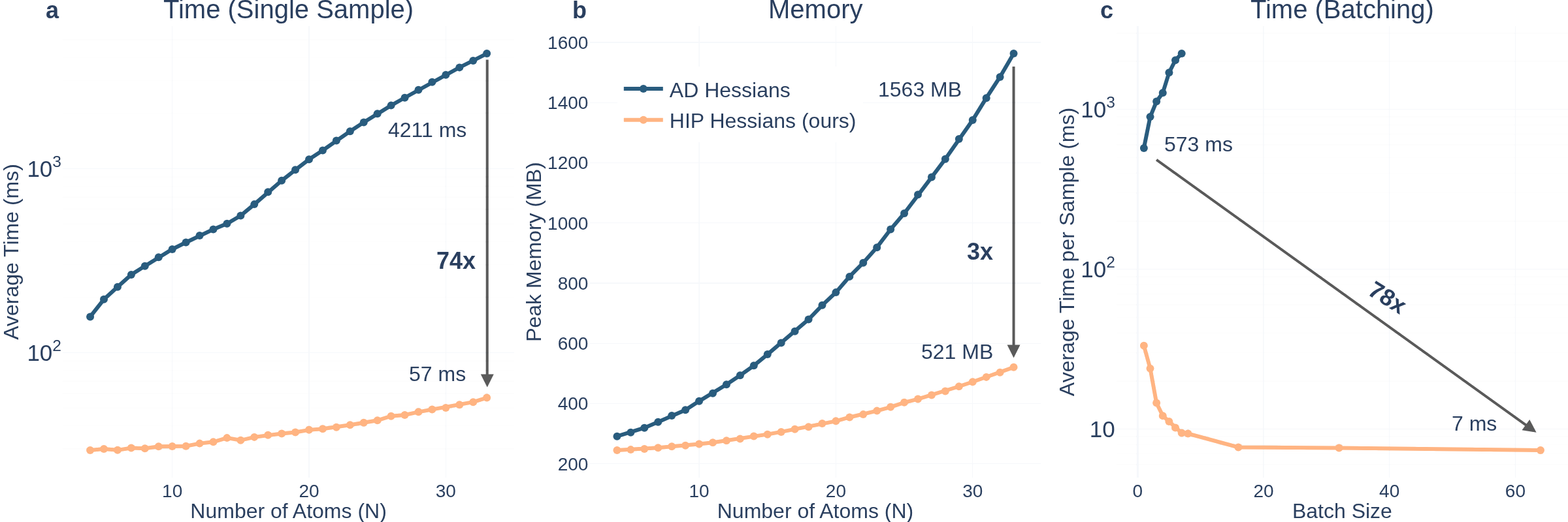
HIP is blanzingly fast. Over 70x faster for a small molecule, with better size scaling!

This speedup is also why HIP is more accurate: it is much cheaper to train.

The failure of autodiff and finite difference

Autodiff and finite difference Hessians are not accurate out of the box, they need special training. But due the high cost of autodiff and finite difference, this means that including them in training is prohibitively expensive.

For example, HORM used multiple GPUs only to be able to include two columns of the Hessian per batch into the loss (random Jacobian-vector products). By comparison, we trained HIP on a single H100 for only three days to get a higher accuracy.

The reason autodiff and finite difference Hessians fail on regular MLIPs seems to be because the forces are not smooth by default. That the forces are not smooth is not surprising. Theoretically one can fit a function well without fitting it’s derivative accurately. Experimentally, just training on the energy also does not give accurate autodiff forces. Brook Wander and colleagues argue that most MLIP data comes from molecular dynamics, with distance between configurations much larger than used during finite difference. They are able to improve the forces by finetuning on configurations with tiny displacements from finite difference DFT Hessians.

From what I can tell, the errors of the finite difference Hessians after finetuning are still a magnitude larger than for HIP. Also, central difference requires 6N forward passes compared to just one with HIP.

Sneak peak: unpublished results

Finally, I want to end with nice result we found since publishing the paper: HIP improves energies and forces across all data scales! All runs were limited to the same wall clock training time of three days to keep it fair. Additionally predicting the Hessian and including it in the loss seems to improve the features learned by the backbone!

MAE [kcal, Ang] with HIP (orange) vs energy and forces only (blue)

I find this result highly encouraging. With HIP we do not just get the Hessian “for free”, we even gain better predictions! This makes me go spend some CPU hours on collecting DFT Hessians, and turn all our MLIPs into HIPs.

This was a team effort between UofT and DTU:
Andreas Burger, Luca Thiede, Nikolaj Rønne, Varinia Bernales, Nandita Vijaykumar, Tejs Vegge, Arghya Bhowmik, Alan Aspuru-Guzik

The full paper and the code are openly available:
Paper: https://arxiv.org/abs/2509.21624
Code: https://github.com/BurgerAndreas/hip

If you have any feedback, questions, or complaints, please write me at:
andreas (dot) burger (at) mail.utoronto.ca

All the best,
Andreas